How Circuitscape Works

Whatever software you use, connectivity modeling involves a great deal of research, data compilation, GIS analyses, and careful interpretation of results. Defining areas to connect, parameterizing resistance models, and other modeling decisions you will need to make are not trivial. Before diving in, we strongly recommend that users first acquaint themselves with the process and challenges of connectivity modeling by consulting published resources. Good places to start include overviews on the Corridor Design and Connecting Landscapes websites. Spear et al. (2010), Beier et al. (2011) and Zeller et al. (2012) offer helpful advice on resistance mapping and connectivity analysis in general. Before using this software, users should acquaint themselves with the use of circuit theory for modeling connectivity (summarized in McRae et al. 2008).

See the Gnarly Landscape Utilities website for tools that can help to automate resistance and core area modeling.

Lastly, users interested in mapping important connectivity areas may wish to consider Linkage Mapper, which maps least-cost corridors. Linkage Mapper now also hybridizes least-cost corridor modeling with Circuitscape (see the Pinchpoint Mapper tool within the Linkage Mapper toolkit). Links to other connectivity tools can be found on the Corridor Design and Connecting Landscapes websites.

Circuitscape may be called through its own graphical user interface, from the Circuitscape for ArcGIS Toolbox, or from the command line. Users supply Circuitscape with resistance data and the program calculates effective resistances and/or creates maps of current flow and voltages across landscapes and networks.

Two data types: network and raster

Circuitscape reads either a network of nodes connected by links or a raster grid of resistances (Fig. 3). Links and raster cells are attributed with resistance values that reflect the degree to which the landscape facilitates or impedes movement. Networks and raster maps can be coded in resistances (with higher values denoting greater resistance to movement) or conductances (the reciprocal of resistance; higher values indicate greater ease of movement).

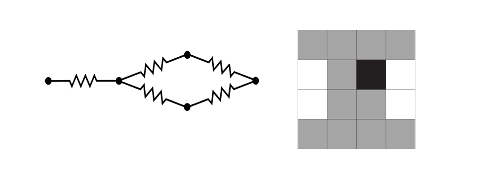
Fig. 1. Simple illustrations of network and raster data types used by Circuitscape. The program can operate on networks of nodes (left panel) or raster grids (right panel). Raster grid cells can have any resistance value. Here, cells with zero resistance ("short-circuit regions," which can be used to represent contiguous habitat patches) are shown in white, cells with a resistance of 1 are shown in gray, and a cell with infinite resistance (coded as NODATA) is shown in black.

For rasters, every grid cell with finite resistance is represented as a node in a graph, connected to either its four first-order or eight first- and second-order neighboring cells. Cells with infinite resistance (zero conductance) are dropped. Habitat patches, or collections of cells, can be assigned zero resistance (infinite conductance) using a separate "short-circuit region" file. These collections of cells are collapsed into a single node.

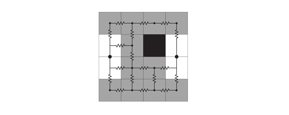
Fig. 2. Raster grids are converted to electrical networks. Each cell becomes a node (represented by a dot), and adjacent cells are connected to their four or eight neighbors by resistors. Here, the two short-circuit regions have each been collapsed into a single node. The infinite resistance cell is dropped entirely from the network.

Calculation modes

Circuitscape operates in one of four modes: pairwise, advanced, one-to-all, and all-to-one. Pairwise and advanced modes are available for both raster and network data types. The one-to-all and all-to-one modes are available for raster data only.

In the pairwise mode, connectivity is calculated between all pairs of focal nodes (points or regions between which connectivity is to be modeled) supplied to the program in a single input file. For each pair of focal nodes, one node will arbitrarily be connected to a 1-amp current source, while the other will be connected to ground. Effective resistances will be calculated iteratively between all pairs of focal nodes, and, if selected, maps of current and voltage will be produced. If there are n focal nodes, there will be n(n - 1)/2 calculations unless you're using focal points (only one cell per focal node) and not mapping currents or voltages. In the latter case, we can do it in n calculations (much faster).

The advanced mode offers much greater flexibility in defining sources and targets for current flow. The user defines any number of current sources and any number of grounds in a network or raster landscape, and these are all activated simultaneously. Sources represent points or areas from which current flows, whereas grounds represent nodes where current exits the system.

Source nodes can have different strengths (i.e. inject more or less current into the network or grid), and ground nodes can be tied to ground with any resistance. Current sources and grounds are supplied in separate input files.

Two other modes are available for raster data types only. The one-to-all mode is similar to the pairwise mode, and takes the same input files. However, instead of iterating across all focal node pairs, this mode iterates across all focal nodes. In each iteration, one focal node is connected to a 1-amp current source, while all remaining focal nodes are connected to ground. If there are n focal nodes, there will be n calculations.

The all-to-one mode is similar to the one-to-all mode, and takes the same input files. However, in this mode Circuitscape connects one focal node to ground and all remaining focal nodes to 1-amp current sources. It then repeats the process for each focal node; if there are n focal nodes, there will be n calculations.

Circuitscape can generate maps showing the current density and voltage at each node or cell under each configuration (and current flow for each link/resistor in networks). Additionally, Circuitscape writes a file reporting effective resistances between all pairs of focal nodes in the pairwise mode, and between each node and ground in the one-to-all mode. Resistances in the all-to-one mode are undefined, so a file is written with zeros indicating successful solves.

Illustrations of analyses with network data

For network data types, any node can be connected to any other node by a resistor:

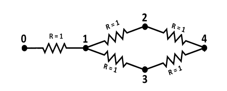
Fig. 3. Example network. This network would be input as a text list specifying resistances between each pair of connected nodes (0-1, 1-2, 1-3, 2-3, and 2-4; see the Input file formats section below).

For pairwise analysis we would also supply a list of focal nodes (containing at least two node numbers, but as many as five, the number of nodes in the circuit) between which we want to perform calculations.

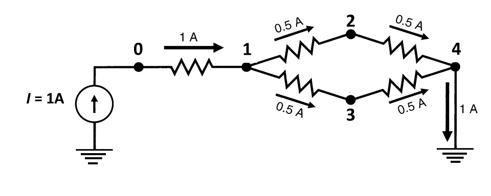
Fig 4. In pairwise mode, Circuitscape will iterate across pairs of nodes in a focal node list. If node 0 and node 4 are in the focal node list, then one of the iterations will look like the above, with a 1 amp current source connected to one node and the other grounded. Current will flow across the network from the source to the ground. Branch currents, node currents, node voltages, and effective resistances between node pairs can be written for each iteration.

More complexity can be added by running in advanced mode, which allows any number of sources and grounds to be activated simultaneously. For example, we could modify the circuit above by adding a single, fixed source at node zero and adding multiple grounds with different resistances. Current sources and grounds are entered in separate files.

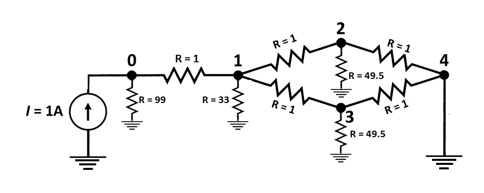
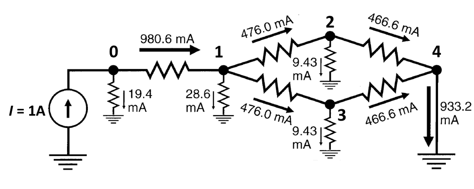
Fig. 5. In advanced mode, any node can be tied to a current source or to ground, either directly or via resistors with any value (top panel). Currents passing through all nodes and links can then be calculated (bottom panel), and voltages can be calculated at each node. Circuit above is from McRae et al. (2008).

Illustrations of analyses with raster data

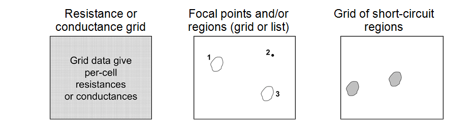
Fig. 6. Example raster input files for pairwise, one-to-all, and all-to-one modes. Input files in this example include a resistance map specifying per-cell resistances or conductances, a focal node location file (with two focal regions and one focal point in this case), and an optional short-circuit region map. Focal regions and short-circuit regions represent areas with zero resistance. Cells with the same region ID are considered perfectly connected and are collapsed into a single node, even if they are not contiguous.

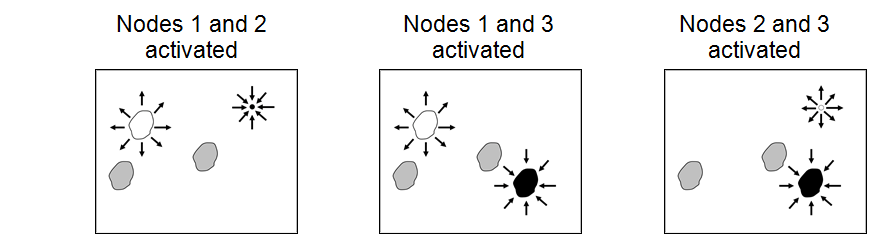
Fig. 7. Schematic describing pairwise mode analyses that would result from the input files shown in Fig. 8. Three sets of pairwise calculations, involving focal nodes 1 and 2, nodes 1 and 3, and nodes 2 and 3, would be conducted. For each pair, one node would be connected to a 1-amp current source, and the other to ground. Note that focal region nodes become short-circuit regions when they are activated (e.g., node 1 in scenario 1), but these regions are not present when the nodes are not activated (e.g., node 1 in scenario 3).

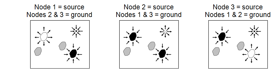
Fig. 8. Schematic describing one-to-all mode analyses that would result from the input files shown in Fig. 8. Three sets of calculations, involving focal nodes 1, 2, and 3, would be conducted. For each, one node would be connected to a 1-amp current source, and the other two would be connected to ground. The all-to-one mode is similar, with arrow directions reversed; that is, one node is connected to ground while the remaining nodes are connected to 1-amp current sources.

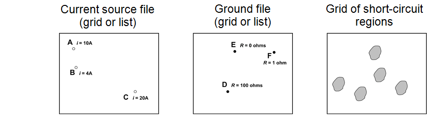
Fig. 9. Example raster input files for advanced mode, which requires independent current source and ground files. Note that current sources in this example have different "strengths," and ground nodes are connected to ground with differing levels of resistance. This example also includes an optional grid with five short-circuit regions.

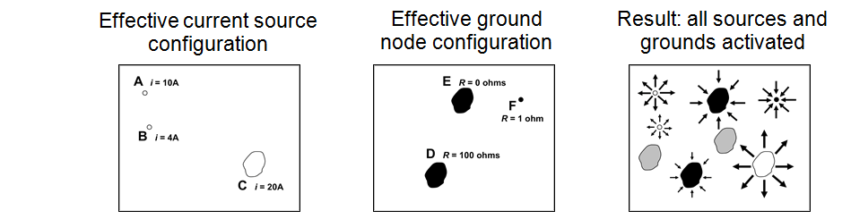
Fig. 10. The first two panels show the "effective" configuration resulting from the input files in Fig. 11. Because current source C and grounds D and E overlap with short-circuit regions, these short-circuit regions effectively become sources or grounds themselves. The rightmost panel shows a schematic of the resulting analysis, with all sources (white points and polygons) and grounds (black points and polygons) activated simultaneously. Note that sources may be negative (drawing current out of the system), and ground nodes can actually contribute current to the system when negative sources are present.