Examples
Forest connectivity in central Maryland
Land cover datasets are commonly used to parameterize resistance for connectivity modeling. This example uses the National Land Cover Dataset for the United States to model forest connectivity in central Maryland. Each value in the categorical land cover dataset is assigned a resistance score. We can have Omniscape.jl assign these values internally by providing a reclassification table (see Resistance Reclassification).
First, install the necessary packages and import them:
using Pkg; Pkg.add(["Omniscape", "Rasters", "Plots"])
using Omniscape, Rasters, Plots
Next, download the landcover data we'll use in this example, and plot it:
url_base = "https://raw.githubusercontent.com/Circuitscape/datasets/main/"
# Download the NLCD tile used to create the resistance surface and load it
download(string(url_base, "data/nlcd_2016_frederick_md.tif"),
         "nlcd_2016_frederick_md.tif")

# Plot the landcover data
values = [11, 21, 22, 23, 24, 31, 41, 42, 43, 52, 71, 81, 82, 90, 95]
palette = ["#476BA0", "#DDC9C9", "#D89382", "#ED0000", "#AA0000",
           "#b2b2b2", "#68AA63", "#1C6330", "#B5C98E", "#CCBA7C",
           "#E2E2C1", "#DBD83D", "#AA7028", "#BAD8EA", "#70A3BA"]

plot(Raster("nlcd_2016_frederick_md.tif"),
     title = "Land Cover Type", xlabel = "Easting", ylabel = "Northing",
     seriescolor = cgrad(palette, (values .- 12) ./ 84, categorical = true),
     size = (700, 640))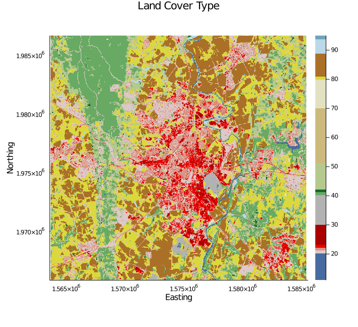
Now, load the array using Omniscape's internal read_raster() function or a function from a GIS Julia package of your choice. read_raster() returns a tuple with the data array, a wkt string containing geographic projection info, and an array containing geotransform values. We'll use the wkt and geotransform later.
land_cover, wkt, transform = Omniscape.read_raster("nlcd_2016_frederick_md.tif", Float64)(Union{Missing, Float64}[82.0 82.0 … 43.0 43.0; 82.0 82.0 … 43.0 43.0; … ; 82.0 81.0 … 82.0 82.0; 81.0 81.0 … 22.0 82.0], "PROJCS[\"Albers_Conical_Equal_Area\",GEOGCS[\"WGS 84\",DATUM[\"WGS_1984\",SPHEROID[\"WGS 84\",6378137,298.257223563,AUTHORITY[\"EPSG\",\"7030\"]],AUTHORITY[\"EPSG\",\"6326\"]],PRIMEM[\"Greenwich\",0],UNIT[\"degree\",0.0174532925199433,AUTHORITY[\"EPSG\",\"9122\"]],AUTHORITY[\"EPSG\",\"4326\"]],PROJECTION[\"Albers_Conic_Equal_Area\"],PARAMETER[\"latitude_of_center\",0],PARAMETER[\"longitude_of_center\",0],PARAMETER[\"standard_parallel_1\",29.5],PARAMETER[\"standard_parallel_2\",45.5],PARAMETER[\"false_easting\",0],PARAMETER[\"false_northing\",0],UNIT[\"metre\",1,AUTHORITY[\"EPSG\",\"9001\"]],AXIS[\"Easting\",EAST],AXIS[\"Northing\",NORTH]]", [1.56369e6, 30.0, 0.0, 1.98666e6, 0.0, -30.0])The next step is to create a resistance reclassification table that defines a resistance value for each land cover value. Land cover values go in the left column, and resistance values go in the right column. In this case, we are modeling forest connectivity, so forest classes receive the lowest resistance score of one. Other "natural" land cover types are assigned moderate values, and human-developed land cover types are assigned higher values. Medium- to high-intensity development are given a value of missing, which denotes infinite resistance (absolute barriers to movement).
# Create the reclassification table used to translate land cover into resistance
reclass_table = [
    11.	100; # Water
    21	500; # Developed, open space
    22	1000; # Developed, low intensity
    23	missing; # Developed, medium intensity
    24	missing; # Developed, high intensity
    31	100; # Barren land
    41	1; # Deciduous forest
    42	1; # Evergreen forest
    43	1; # Mixed forest
    52	20; # Shrub/scrub
    71	30; # Grassland/herbaceous
    81	200; # Pasture/hay
    82	300; # Cultivated crops
    90	20; # Woody wetlands
    95	30; # Emergent herbaceous wetlands
]
15×2 Matrix{Union{Missing, Float64}}:
11.0 100.0
21.0 500.0
22.0 1000.0
23.0 missing
24.0 missing
31.0 100.0
41.0 1.0
42.0 1.0
43.0 1.0
52.0 20.0
71.0 30.0
81.0 200.0
82.0 300.0
90.0 20.0
95.0 30.0Next, we define the configuration options for this model run. See the Settings and Options section in the User Guide for more information about each of the configuration options.
# Specify the configuration options
config = Dict{String, String}(
    "radius" => "100",
    "block_size" => "21",
    "project_name" => "md_nlcd_omniscape_output",
    "source_from_resistance" => "true",
    "r_cutoff" => "1", # Only forest pixels should be sources
    "reclassify_resistance" => "true",
    "calc_normalized_current" => "true",
    "calc_flow_potential" => "true"
)
Dict{String, String} with 8 entries:
"calc_normalized_current" => "true"
"calc_flow_potential" => "true"
"radius" => "100"
"source_from_resistance" => "true"
"block_size" => "21"
"r_cutoff" => "1"
"project_name" => "md_nlcd_omniscape_output"
"reclassify_resistance" => "true"Finally, compute connectivity using run_omniscape(), feeding in the configuration dictionary, the resistance array, the reclass table, as well as the wkt and geotransform information loaded earlier. Passing in the wkt and geotransform, along with true for the write_outputs argument, will allow Omniscape to write the outputs as properly projected rasters. run_omniscape will print some information to the console and show progress, along with an ETA, in the form of a progress bar.
currmap, flow_pot, norm_current = run_omniscape(config,
                                                land_cover,
                                                reclass_table = reclass_table,
                                                wkt = wkt,
                                                geotransform = transform,
                                                write_outputs = true)
(Union{Missing, Float64}[0.0027258956360456245 0.00949946238540265 … 0.7701753044818226 0.5588858207982137; 0.008791599816740273 0.01685623544448697 … 1.1963152183457204 0.8100820554386359; … ; 0.22307355874067347 0.621662091061402 … 0.9836258338404573 0.443012935545784; 0.06824326358051583 0.12451438738405202 … 0.3755969475119765 0.13747736528383855], Union{Missing, Float64}[0.22851654463598325 0.7582581265070772 … 0.8429397856671239 0.5590075422826746; 0.7733371879936655 1.3188749872253167 … 1.2799958538141314 0.7890368128348983; … ; 0.13214272974421676 0.23699796618096516 … 0.4059086986242947 0.2336255195256739; 0.04552497135409578 0.1525431391804039 … 0.23018154785287886 0.06914308189257573], Union{Missing, Float64}[0.011928657683792024 0.012528006035572617 … 0.913677723578187 0.9997822543074038; 0.011368391373430611 0.012780768160558988 … 0.9346242917748058 1.026672066830602; … ; 1.6881258558262553 2.623069307635821 … 2.423268673901695 1.89625232913436; 1.4990292481397935 0.8162568834826198 … 1.6317422096407148 1.988302539036812])You'll see that outputs are written to a new folder called "md_nlcd_omniscape_output". This is specified by the "project_name" value in config above. The cumulative current map will always be called "cum_currmap.tif", and it will be located in the output folder. We also specified in the run configuration that flow potential and normalized current should be computed as well. These are called "flow_potential.tif" and "normalized_cum_currmap.tif", respectively. See Outputs for a description of each of these outputs.
Now, plot the outputs. Load the outputs into Julia as spatial data and plot them.
First, the cumulative current map:
current = Raster("md_nlcd_omniscape_output/cum_currmap.tif")
plot(current,
     title = "Cumulative Current Flow", xlabel = "Easting", ylabel = "Northing",
     seriescolor = cgrad(:inferno, [0, 0.005, 0.03, 0.06, 0.09, 0.14]),
     size = (600, 550))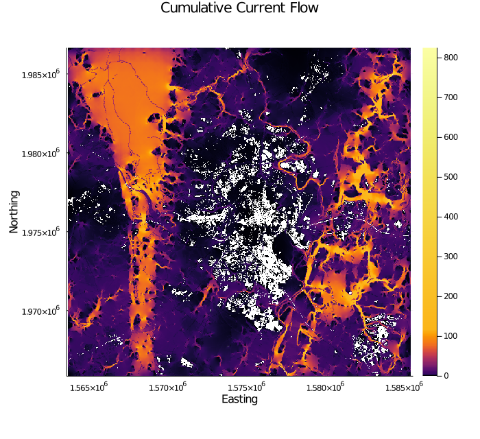
Cumulative current flow representing forest connectivity. Note that areas in white correspond to built up areas (NLCD values of 23 and 24) that act as absolute barriers to movement.
Next, flow potential. This map shows what connectivity looks like under "null" conditions (resistance equals 1 for the whole landscape).
fp = Raster("md_nlcd_omniscape_output/flow_potential.tif")
plot(fp,
     title = "Flow Potential", xlabel = "Easting", ylabel = "Northing",
     seriescolor = cgrad(:inferno, [0, 0.005, 0.03, 0.06, 0.09, 0.14]),
     size = (700, 640))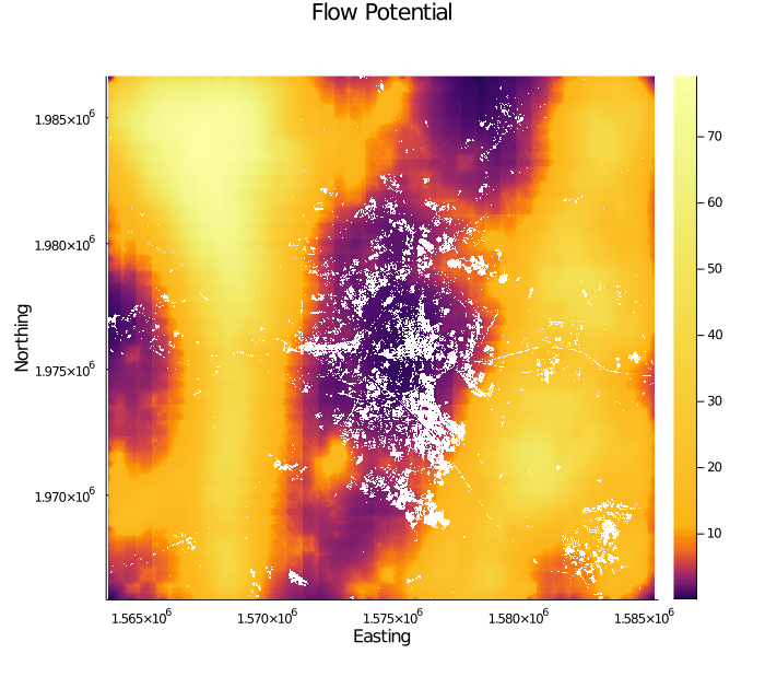
Flow potential, which shows what connectivity would look like in the absence of barriers to movement. The blocking that you can see is an artifact of setting a large block_size to make the example run faster. Set a smaller block_size to reduce/remove this issue.
Finally, map normalized current flow, which is calculated as cumulative current divided by flow potential.
normalized_current = Raster("md_nlcd_omniscape_output/normalized_cum_currmap.tif")
plot(normalized_current,
     title = "Normalized Current Flow", xlabel = "Easting", ylabel = "Northing",
     seriescolor = cgrad(:inferno, [0, 0.005, 0.03, 0.06, 0.09, 0.14]),
     size = (700, 640))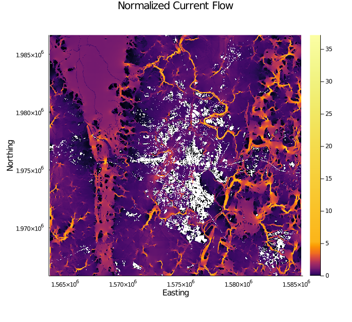
Normalized cumulative current. Values greater than one indicate areas with channelized/bottlenecked flow. Values around 1 (cumulative current ≈ flow potential) indicate diffuse current. Values less than 1 indicate impeded flow.