Examples
Habitat Corridor Mapping
In this example, we'll map a habitat corridor in central Maryland. We'll use SpatialGraphs.jl to convert the landscape into a graph, then calculate cost distances, and finally convert the result back into a raster to display a least cost corridor in space.
First, install the necessary packages and import them:
using Pkg
Pkg.add(["Rasters", "Plots", "Graphs", "SimpleWeightedGraphs", "SpatialGraphs"])
using SpatialGraphs, Rasters, Plots, Graphs, SimpleWeightedGraphs
Now, let's download the land cover map that we'll use as the basis for defining the weights of our graph, and plot it. Graph weights correspond to the cost of an animal moving from one graph vertex to another. This is also commonly referred to as "resistance" in the context of connectivity modeling.
url_base = "https://raw.githubusercontent.com/Circuitscape/datasets/main/"
download(string(url_base, "nlcd_2016_frederick_md.tif"),
         "nlcd_2016_frederick_md.tif")
values = [11, 21, 22, 23, 24, 31, 41, 42, 43, 52, 71, 81, 82, 90, 95]
palette = ["#476BA0", "#DDC9C9", "#D89382", "#ED0000", "#AA0000",
           "#b2b2b2", "#68AA63", "#1C6330", "#B5C98E", "#CCBA7C",
           "#E2E2C1", "#DBD83D", "#AA7028", "#BAD8EA", "#70A3BA"]

plot(Raster("nlcd_2016_frederick_md.tif"), title = "Land Cover Type",
     xlabel = "Easting", ylabel = "Northing",
     seriescolor = cgrad(palette, (values .- 12) ./ 84,
     categorical = true), size = (700, 640))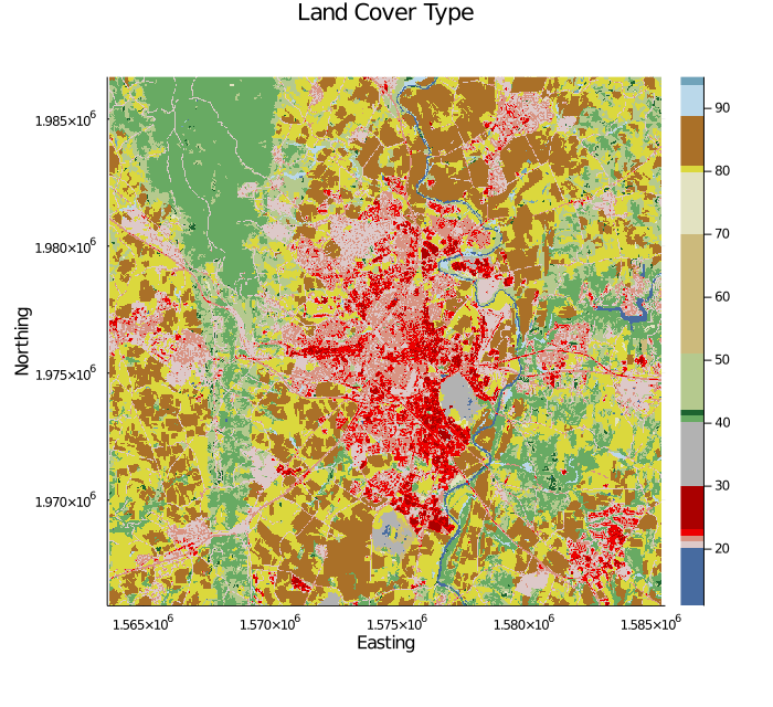
Load the land cover data as a Raster, read it into memory, then convert it to Float64.
landcover = convert.(
    Float64,
    read(
        Raster(
            "nlcd_2016_frederick_md.tif",
            missingval = -9999.0
        )
    )
)
725×694×1 Raster{Float64,3} with dimensions:
X Projected range(1.56369e6, stop=1.58541e6, length=725) ForwardOrdered Regular Intervals crs: WellKnownText,
Y Projected range(1.98663e6, stop=1.96584e6, length=694) ReverseOrdered Regular Intervals crs: WellKnownText,
Band Categorical 1:1 ForwardOrdered
with missingval: -9999.0
[:, :, 1]
82.0 82.0 82.0 82.0 82.0 41.0 … 81.0 81.0 81.0 82.0 82.0 81.0
82.0 82.0 82.0 82.0 82.0 41.0 82.0 82.0 82.0 82.0 81.0 81.0
82.0 82.0 82.0 82.0 41.0 41.0 82.0 82.0 82.0 82.0 81.0 43.0
82.0 82.0 82.0 82.0 82.0 41.0 82.0 82.0 82.0 82.0 82.0 81.0
82.0 82.0 82.0 82.0 82.0 41.0 82.0 82.0 82.0 82.0 82.0 81.0
82.0 82.0 82.0 82.0 82.0 41.0 … 82.0 82.0 82.0 82.0 82.0 81.0
⋮ ⋮ ⋱ ⋮
43.0 43.0 43.0 43.0 43.0 81.0 82.0 22.0 21.0 81.0 81.0 43.0
43.0 43.0 43.0 43.0 43.0 43.0 … 82.0 82.0 22.0 21.0 81.0 81.0
43.0 43.0 43.0 43.0 43.0 43.0 82.0 82.0 22.0 22.0 21.0 43.0
43.0 43.0 43.0 43.0 43.0 43.0 22.0 82.0 82.0 82.0 22.0 21.0
43.0 43.0 43.0 43.0 43.0 81.0 82.0 82.0 82.0 82.0 82.0 22.0
43.0 43.0 43.0 43.0 81.0 81.0 82.0 82.0 82.0 82.0 82.0 82.0Now, we need to convert land cover into resistance by reclassifying the values in the land cover raster to their corresponding costs/weights.
# Copy the landcover object to use as a place holder for resistance
resistance = deepcopy(landcover)

# Define how values should be reclassified. Original values are on the left,
# and new values are on the right.
reclass_table = [
    11.	100; # Water
    21	500; # Developed, open space
    22	1000; # Developed, low intensity
    23	-9999; # Developed, medium intensity
    24	-9999; # Developed, high intensity
    31	100; # Barren land
    41	1; # Deciduous forest
    42	1; # Evergreen forest
    43	1; # Mixed forest
    52	20; # Shrub/scrub
    71	30; # Grassland/herbaceous
    81	200; # Pasture/hay
    82	300; # Cultivated crops
    90	20; # Woody wetlands
    95	30; # Emergent herbaceous wetlands
]

# Redefine the values in resistance based on the corresponding land cover
# values, using reclass_table
for i in 1:(size(reclass_table)[1])
    resistance[landcover .== reclass_table[i, 1]] .= reclass_table[i, 2]
end
Now that we have a resistance raster, we can start using SpatialGraphs.jl!
Convert the resistance raster into a WeightedRasterGraph:
wrg = weightedrastergraph(resistance)WeightedRasterGraph{Int64, Float64}:
graph: SimpleWeightedGraphs.SimpleWeightedGraph{Int64, Float64} with 472395 vertices and 1842168 edges
vertex_raster: Raster{Int64, 3} with dimensions:
X: range(1.56369e6, 1.58541e6, step=30.0)
Y: range(1.96584e6, 1.98663e6, step=-30.0)
Band: 1:1Now that we have a WeightedRasterGraph, we can make use of the functions in Graphs.jl.
Let's calculate cost distances from two different vertices. Vertex IDs, the second argument to dijkstra_shortest_paths, correspond to the values in wrg.vertex_raster.
First, we'll use dijkstra_shortest_paths to calculate to total cost distance from each vertex of interest to all other vertices in the graph.
cd_1 = dijkstra_shortest_paths(wrg, 1)
cd_2 = dijkstra_shortest_paths(wrg, 348021)
Graphs.DijkstraState{Float64, Int64}([718, 718, 719, 5, 6, 723, 723, 724, 8, 11 … 471667, 471669, 471669, 471670, 471671, 472390, 471673, 471675, 471675, 471676], [25701.62603007754, 25577.361961365612, 25515.02282022846, 25278.70510711612, 24978.70510711612, 24678.70510711612, 24566.365965978966, 24466.451752416593, 24566.951752416593, 24565.709111729473 … 10062.751906195092, 10065.272900944012, 9982.430188469392, 9978.87679787612, 9917.037656738969, 10017.537656738969, 10003.812439463301, 9929.048370751374, 10013.362945802135, 9601.023804664985], [Int64[], Int64[], Int64[], Int64[], Int64[], Int64[], Int64[], Int64[], Int64[], Int64[] … Int64[], Int64[], Int64[], Int64[], Int64[], Int64[], Int64[], Int64[], Int64[], Int64[]], [4.0298935876110776e136, 1.3432978625370258e136, 1.3432978625370258e136, 1.4160598300911148e137, 1.4160598300911148e137, 1.4160598300911148e137, 1.4160598300911148e137, 8.496358980546688e136, 8.496358980546688e136, 7.365264750938306e135 … 1.7619493254311218e33, 1.006828185960641e33, 2.5170704649016025e32, 2.5170704649016025e32, 2.5170704649016025e32, 2.5170704649016025e32, 3.020484557881923e33, 1.006828185960641e33, 1.006828185960641e33, 1.006828185960641e33], Int64[])Now, create placeholder rasters to store the cost distance values for each vertex, and populate them using the cost distances calculated above. Finally, we'll sum the rasters to enable us to delineate a corridor. The value at each pixel corresponds to the total cost distance of the least cost path between vertices 1 and 348021 that intersects that pixel.
# Create rasters
cd_1_raster = Raster( # Start with an empty raster that will be populated
    fill(float(resistance.missingval), size(wrg.vertex_raster)),
    dims(resistance),
    missingval=resistance.missingval
)
cd_2_raster = Raster(
    fill(float(wrg.vertex_raster.missingval), size(wrg.vertex_raster)),
    dims(resistance),
    missingval=resistance.missingval
)

# Populate with cost distances
cd_1_raster[wrg.vertex_raster .!= wrg.vertex_raster.missingval] .= cd_1.dists[
    wrg.vertex_raster[wrg.vertex_raster.!= wrg.vertex_raster.missingval]
]
cd_2_raster[wrg.vertex_raster .!= wrg.vertex_raster.missingval] .= cd_2.dists[
    wrg.vertex_raster[wrg.vertex_raster.!= wrg.vertex_raster.missingval]
]

# Sum the rasters to enalbe corridor mapping
cwd_sum = cd_1_raster + cd_2_raster
725×694×1 Raster{Float64,3} with dimensions:
X Projected range(1.56369e6, stop=1.58541e6, length=725) ForwardOrdered Regular Intervals crs: WellKnownText,
Y Projected range(1.98663e6, stop=1.96584e6, length=694) ReverseOrdered Regular Intervals crs: WellKnownText,
Band Categorical 1:1 ForwardOrdered
with missingval: -9999.0
[:, :, 1]
25701.6 25701.6 25701.6 25814.9 … 73534.8 74034.8 74634.8 75134.8
25877.4 25701.6 25701.6 25701.6 73841.9 74241.9 74741.9 75141.9
26115.0 25939.3 25763.6 25763.6 74290.4 74690.4 74949.0 75026.1
26178.7 26240.6 26125.9 25950.2 74608.8 75138.9 75449.0 75227.1
26178.7 26240.6 26363.9 26486.0 74857.3 75457.3 75934.3 75627.1
26136.5 26011.8 26009.8 26007.8 … 75105.9 75705.9 76305.9 76027.1
⋮ ⋱ ⋮
39101.2 39099.2 39097.2 39095.2 44093.3 44793.3 45193.3 45394.3
39100.4 39098.4 39096.4 39094.4 … 44261.9 45493.3 45359.0 45595.3
39099.5 39097.5 39095.5 39093.5 44261.1 45174.0 45066.9 45567.9
39098.7 39096.7 39094.7 39092.7 43335.5 43935.5 45235.5 45418.3
39099.5 39097.5 39095.5 39093.5 43087.0 43687.0 44287.0 45587.0
39100.4 39098.4 39096.4 39094.4 42962.3 43562.3 44162.3 44762.3Setting some land cover classes to NoData resulted in some vertices being completely isolated from the vertices from which we calculated cost distances above. In these cases, dijkstra_shortest_paths returns a value of Inf for the cost distance. Let's get rid of those by setting them to the NoData value of our raster.
cwd_sum[cwd_sum .== Inf] .= cwd_sum.missingval1340-element view(::Array{Float64, 3}, CartesianIndex{3}[CartesianIndex(525, 46, 1), CartesianIndex(494, 65, 1), CartesianIndex(384, 144, 1), CartesianIndex(384, 145, 1), CartesianIndex(287, 151, 1), CartesianIndex(287, 152, 1), CartesianIndex(287, 153, 1), CartesianIndex(352, 165, 1), CartesianIndex(424, 168, 1), CartesianIndex(425, 168, 1) … CartesianIndex(609, 630, 1), CartesianIndex(653, 641, 1), CartesianIndex(666, 641, 1), CartesianIndex(242, 665, 1), CartesianIndex(245, 665, 1), CartesianIndex(246, 665, 1), CartesianIndex(247, 665, 1), CartesianIndex(248, 665, 1), CartesianIndex(246, 666, 1), CartesianIndex(247, 666, 1)]) with eltype Float64:
-9999.0
-9999.0
-9999.0
-9999.0
-9999.0
-9999.0
-9999.0
-9999.0
-9999.0
-9999.0
⋮
-9999.0
-9999.0
-9999.0
-9999.0
-9999.0
-9999.0
-9999.0
-9999.0
-9999.0Finally, let's plot the result! We'll use a threshold to set pixels above a certain value to NoData, so we will only retain the pixels within our "corridor".
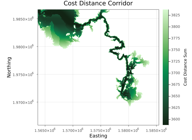
corridor = copy(cwd_sum)
corridor[cwd_sum .>= (minimum(cwd_sum[cwd_sum .>= 0]) + 250)] .= -9999

plot(
    cwd_sum,
    title = "Cost Distance Corridor",
    xlabel = "Easting", ylabel = "Northing",
    colorbar_title = " \nCost Distance Sum",
    size = (650, 475)
)